|
|
Copyright
This work is copyright 2010 by Joshua J. Cogliati. This work is licensed under the Creative Commons Attribution 3.0 Unported License. To view a copy of this license, visit http://creativecommons.org/licenses/by/3.0/ or send a letter to Creative Commons, 171 Second Street, Suite 300, San Francisco, California, 94105, USA. As specified in the license, verbatim copying and use is freely permitted, and properly attributed use is also allowed.
Committee Approval Page
To the graduate faculty:
The members of the Committee appointed to examine the thesis of Joshua J. Cogliati find it satisfactory and recommend that it be accepted.
___________________________
Dr. Abderrafi M. Ougouag,
Major Advisor, Chair
_____________________________
Dr. Mary Lou Dunzik-Gougar,
Co-Chair
_____________________________
Dr. Michael Lineberry,
Committee Member
_____________________________
Dr. Steve C. Chiu,
Committee Member
_____________________________
Dr. Steve Shropshire,
Graduate Faculty Representative
Acknowledgments
Thanks are due to many people who have provided information, comments and insight. I apologize in advance for anyone that I have left out. The original direction and technical ideas came from my adviser Abderrafi Ougouag as well as continued encouragement and discussion throughout its creation. Thanks go to Javier Ortensi for the encouragement and discussion as he figured out how use the earthquake data and I figured out how to generate it. At INL the following people assisted: Rob Bratton and Will Windes with the graphite literature review, Brian Boer with discussion and German translation, Hongbin Zhang with encouragement and Chinese translation and Suzette J. Payne for providing me with the Earthquake motion data. The following PBMR (South Africa) employees provided valuable help locating graphite literature and data: Frederik Reitsma, Pieter Goede and Alastair Ramlakan. The Juelich (Germany) people Peter Pohl, Johannes Fachinger and Werner von Lensa provided valuable assistance with understanding AVR. Thanks to Professor Mary Dunzik-Gougar for introducing me to many of these people, as well as encouragement and feedback on this PhD and participating as co-chair on the dissertation committee. Thanks to the other members of my committee, Dr. Michael Lineberry, Dr. Steve C. Chiu and Dr. Steve Shropshire, for providing valuable feedback on the dissertation. Thanks to Gannon Johnson for pointing out that length needed to be tallied separately from the length times force tally for the wear calculation (this allowed the vibration issue to be found). Thanks to Professor Jan Leen Kloosterman of the Delft University of Technology for providing me the PEBDAN program used for calculating Dancoff factors. The work was partially supported by the U.S. Department of Energy, Assistant Secretary for the office of Nuclear Energy, under DOE Idaho Operations Office Contract DEAC07-05ID14517. The financial support is gratefully acknowledged.
This dissertation contains work that was first published in the following conferences: Mathematics and Computation, Supercomputing, Reactor Physics and Nuclear and Biological Applications, Palais des Papes, Avignon, France, September 12-15, 2005; HTR2006: 3rd International Topical Meeting on High Temperature Reactor Technology October 1-4, 2006, Johannesburg, South Africa; Joint International Topical Meeting on Mathematics & Computation and Supercomputing in Nuclear Applications (M&C + SNA 2007) Monterey, California, April 15-19, 2007; Proceedings of the 4th International Topical Meeting on High Temperature Reactor Technology, HTR2008, September 28-October 1, 2008, Washington, DC USA and PHYSOR 2010 - Advances in Reactor Physics to Power the Nuclear Renaissance Pittsburgh, Pennsylvania, USA, May 9-14, 2010.
My mother helped me edit papers I wrote in my pre-college years, and my father taught me that math is useful in the real world. For this and all the other help in launching me into the world, I thank my parents.
Last, but certainly not least, thanks go to my wife, Elizabeth Cogliati for her encouragement and support. This support has provided me with the time needed to work on the completion of this dissertation. This goes above and beyond the call of duty since I started a PhD the same time we started a family. Thanks to my son for letting my skip my first Nuclear Engineering exam by being born, as well as asking all the really important questions. Thanks to my daughter for working right beside me on her dissertation on the little red toy laptop.
Pebble bed reactors (PBR) have moving graphite fuel pebbles. This unique feature provides advantages, but also means that simulation of the reactor requires understanding the typical motion and location of the granular flow of pebbles.
This dissertation presents a method for simulation of motion of the pebbles in a PBR. A new mechanical motion simulator, PEBBLES, efficiently simulates the key elements of motion of the pebbles in a PBR. This model simulates gravitational force and contact forces including kinetic and true static friction. It’s used for a variety of tasks including simulation of the effect of earthquakes on a PBR, calculation of packing fractions, Dancoff factors, pebble wear and the pebble force on the walls. The simulator includes a new differential static friction model for the varied geometries of PBRs. A new static friction benchmark was devised via analytically solving the mechanics equations to determine the minimum pebble-to-pebble friction and pebble-to-surface friction for a five pebble pyramid. This pyramid check as well as a comparison to the Janssen formula was used to test the new static friction equations.
Because larger pebble bed simulations involve hundreds of thousands of pebbles and long periods of time, the PEBBLES code has been parallelized. PEBBLES runs on shared memory architectures and distributed memory architectures. For the shared memory architecture, the code uses a new O(n) lock-less parallel collision detection algorithm to determine which pebbles are likely to be in contact. The new collision detection algorithm improves on the traditional non-parallel O(n log(n)) collision detection algorithm. These features combine to form a fast parallel pebble motion simulation.
The PEBBLES code provides new capabilities for understanding and optimizing PBRs. The PEBBLES code has provided the pebble motion data required to calculate the motion of pebbles during a simulated earthquake. The PEBBLES code provides the ability to determine the contact forces and the lengths of motion in contact. This information combined with the proper wear coefficients can be used to determine the dust production from mechanical wear. These new capabilities enhance the understanding of PBRs, and the capabilities of the code will allow future improvements in understanding.
Pebble bed nuclear reactors are a unique reactor type that have been proposed and used experimentally. Pebble bed reactors were initially developed in Germany in the 1960s when the AVR demonstration reactor was created. The 10 megawatt HTR-10 reactor achieved first criticality in 2000 in China and future reactors are planned. In South Africa, Pebble Bed Modular Reactor Pty. Ltd. was designing a full scale pebble bed reactor to produce process heat or electricity.
Pebble bed nuclear reactors use graphite spheres (usually about 6 cm in diameter) for containing the fuel of the reactor. The graphite spheres encase smaller spheres of TRistructural-ISOtropic (TRISO) particle fuel. Unlike most reactors, the fuel is not placed in an orderly static arrangement. Instead, the graphite spheres are dropped into the top of the reactor, travel randomly down through the reactor core, and are removed from the bottom of the reactor. The pebbles are then possibly recirculated depending on the amount of burnup of the pebble and the reactor’s method of operation.
The first pebble bed reactor was conceived in 1950s in the West Germany using helium gas-cooling and spherical graphite fuel elements. Construction on the Arbeitsgemeinschaft Versuchsreaktor (AVR) 15 MWe reactor was started in 1959 at the KFA Research Centre Jülich. It started operation in 1967 and continued operation for 21 years until 1988. The reactor operated with an outlet temperature of 950C. The AVR demonstrated the potential for the pebble bed reactor concept. Over the course of its operation, loss-of-coolant experiments were successfully performed.
The second pebble bed reactor was the Thorium High Temperature Reactor (THTR). This reactor was built in West Germany for an electric utility. It was a 300 MWe plant that achieved full power in September 1986. In October 1988, when the reactor was shutdown for maintenance, 35 bolt heads were found in the hot gas ducts leading to the steam generators. The determination was made that the plant could be restarted, but funding difficulties prevented this from occurring and the reactor was decommissioned (Goodjohn, 1991).
The third pebble bed reactor to be constructed and the only one that is currently operable is the 10 MWt High Temperature Reactor (HTR-10). This reactor is at the Tsinghua University in China. Construction was started in 1994 and reached first criticality in December 2000. This reactor is helium cooled and has an outlet temperature of 700C (Wu et al., 2002; Xu and Zuo, 2002).
The use of high temperature helium cooled graphite moderated reactors with TRISO fuel particles have a number of advantages. A TRISO particle consists of spherical fuel kernel (such as uranium oxide) surrounded by four concentric layers: 1) a porous carbon buffer layer to accommodate fission product gases which limits pressure on the outer layers, 2) an interior pyrolytic carbon layer, 3) a layer of silicon carbide, and 4) an outer layer of pyrolytic carbon. The pyrolytic layers shrink and creep with irradiation, partially offsetting the pressure from the fission products in the interior as well as helping contain the fission gases. The silicon carbide acts as a containment mechanism for the metallic fission products.(Miller et al., 2002) These layers provide an in-core containment structure for the radioactive fuel and fission products.
The high temperature gas reactors have some advantages over conventional light water reactors. First, the higher outlet temperatures allow higher Carnot efficiency to be obtained1 . Second, the higher temperatures can be used for process heat, which can reduce the use of methane. Third, the high temperature under which TRISO particles can operate allows for the exploitation of the negative temperature coefficient to safely shutdown the reactor without use of control rods.2 Fourth, the higher temperature is above the annealing temperature for graphite, which safely removes Wigner energy3 . These are advantages of both prismatic and pebble bed high temperature reactors.(Gougar et al., 2004; Wu et al., 2002)
Pebble bed reactors, unlike most other reactors types, have moving fuel. This provides advantages but complicates modeling the reactors. A key advantage is that pebble bed reactors can be refueled online, that is, reactor shutdown is not needed for refueling. As a consequence, the reactors have low excess reactivity, as new pebbles can be added or excess pebbles removed to maintain the reactor at critical. The low excess reactivity removes the need for burnable poisons. A final advantage is that the moving fuel allows the pebble bed to be run with optimal moderation, where both increases and decreases in the fuel-to-moderator ratio cause reduction in reactivity. Ougouag et al. (2004) discuss the advantages of optimal moderation including improved fuel utilization. However, because the fuel is moving, many traditional methods of modeling nuclear reactors are inapplicable without a method for quantifying the motion. Hence, there is a need for development of methods usable for pebble bed reactor modeling.
This dissertation describes a computer code, PEBBLES, that is designed to provide a method of simulating the motion of the pebbles in a pebble bed reactor.
Chapter 4 provides the details of how the simulation works. Chapter 5 has a new static friction model developed for this dissertation.
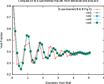
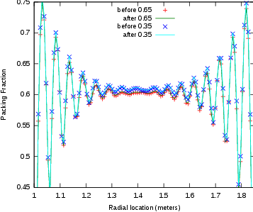
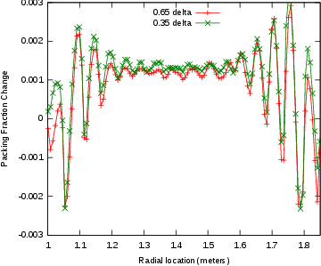
Several checks have been made of the code. Figure 3.1 compares the PEBBLES simulation to experimentally determined radial packing fractions. Section 5.1 describes a new analytical benchmark that was used to test the static friction model in PEBBLES. Section 5.2 uses the Janssen model to test the static friction in a cylindrical vat.
Motivating all the above are the new applications, including Dancoff factors (8.1.1), calculating the angle of repose (8.1.2) and modeling an earthquake in section 8.2.
Most nuclear reactors have fixed fuel, including typical light water reactors. Some reactor designs, such as non-fixed fuel molten salt reactors, have fuel that is in fluid flow. Most designs for pebble bed reactors, however, have moving granular fuel. Since this fuel is neither fixed nor easily treatable as a fluid, predicting the behavior of the reactor requires the ability to understand the characteristics of the positions and motion of the pebbles. For example, predicting the probability of a neutron leaving one TRISO’s fueled region and entering another fueled region depends on the typical locations of the pebbles. A second example is predicting the effect of an earthquake on the reactivity of the pebble bed reactor. This requires knowing how the positions of the pebbles in the reactor change from the forces of the earthquake. Accurate prediction of the typical features of the flow and arrangement of the pebbles in the pebble bed reactor would be highly useful for their design and operation.
The challenge is to gain the ability to predict the pebble flow and pebble positions for start-up, steady state and transient pebble bed reactor operation.
The objective of the research presented in this dissertation is to provide this predicting ability. The approach used is to create a distinct element method computer simulation. The simulation determines the locations and velocities of all the pebbles in a pebble bed reactor and can calculate needed tallies from this data. Over the course of creating this simulation, various applications of the simulation were performed. These models allow the operation of the pebble bed reactor to be better understood.
Because the purpose of this dissertation is to produce a high fidelity simulation that can provide predictions of the pattern and flow of pebbles, previous efforts to simulate granular methods and packing were examined. A variety of simulations of the motion of discrete elements have been created for different purposes. Lu et al. (2001) applied a discrete element method (DEM) to determine the characteristics of packed beds used as fusion reactor blankets. Jullien et al. (1992) used a DEM to determine packing fractions for spheres using different non-motion methods. Soppe (1990) used a rain method to determine pore structures in different sized spheres. The rain method randomly chooses a horizontal position, and then lowers a sphere down until it reaches other existing spheres. This is then repeated to fill up the container. Freund et al. (2003) used a rain method for fluid flow in chemical processing.
The use of non-motion pebble packing methods provide an approximation of the positions of the pebble. Unfortunately, non-motion methods will tend to either under pack or over pack (sometimes both in the same model). For large pebble bed reactors, the approximately ten-meter height of the reactor core will result in different forces at the bottom than at the top. This will change the packing fractions between the top and the bottom, so without key physics, including static friction and the transmittal of force, non-motion physics models will not even be able to get correct positional information. Non-physics based modeling can not be used for predicting the effect of changes in static friction or pebble loading methods even if only the position data is required.
The initial PEBBLES code for calculation of pebble positions minimized the sum of the gravitational and Hookes’ law potential energies by adjusting pebble positions. However, that simulation was insufficient for determining flow and motion parameters and simulation of earthquake packing.
Additional references addressing full particle motion simulation were evaluated. Kohring (1995) created a 3-D discrete element method simulation to study diffusional mixing and provided detailed information on calculating the kinetic forces for the simulation. The author describes a simple method of calculating static friction. Haile (1997) discusses both how to simulate hard spheres and soft spheres using only potential energy. The soft sphere method in Haile proved useful for determining plausible pebble positions, but is insufficient for modeling the motion. Hard spheres are simulated by calculating the collision results from conservation laws. Soft spheres are simulated by allowing small overlaps, and then having a resulting force dependent on the overlap. Soft spheres are similar to what physically happens, in that the contact area distorts, allowing distant points to approach closer than would be possible if the spheres were truly infinitely hard and only touched at one infinitesimal point. Hard spheres are impractical for a pebble bed due to the frequent and continuous contact between spheres so soft spheres are used instead. The dissertation by Ristow (1998) describes multiple methods for simulation of granular materials. On Ristow’s list of methods was a model similar to that used as the kernel of the work supporting this dissertation. Ristow’s dissertation mentioned static friction and provided useful references that will be discussed in Section 3.2.
To determine particle flows, Wait (2001) developed a discrete element method that included only dynamic friction. Concurrently with this dissertation research, Rycroft et al. (2006b) used a discrete element method, created for other purposes, to simulate the flow of pebbles through a pebble bed reactor.
Multiple other discrete element codes have been created and PEBBLES is similar to several of the full motion models. For most of the applications discussed in this dissertation, only a model that simulates the physics with high fidelity is useful. The PEBBLES dynamic friction model is similar to the model used by Wait or Rycroft, but the static friction model incorporates some new improvements that will be discussed later.
In addition to simulation by computer, other methods of determining the properties of granular fluids have been used. Bedenig et al. (1968) used a scale model to experimentally determine residence spectra (the amount of time that pebbles from a given group take to pass through a reactor) for different exit cone angles. Kadak and Bazant (2004) used scale models and small spheres to estimate the flow of pebbles through a full scale pebble bed reactor. These researchers also examined the mixing that would occur between different radial zones as the pebbles traveled downward. Bernal et al. (1960) carefully lowered steel spheres into cylinders and shook the cylinders to determine both loose and dense packing fractions. The packing fraction and boundary density fluctuations were experimentally measured by Benenati and Brosilow (1962). The Benenati and Brosilow data have been used to verify that the PEBBLES code was producing correct boundary density fluctuations (See Figure 3.1). Many experiments were performed in the designing and operating of the AVR reactor to determine relevant properties such as residence times and optimal chute parameters (Bäumer et al., 1990). These experiments provide data for testing the implementation of any computational model of pebble flow.
The PEBBLES simulation uses elements from a number of sources and uses standard classical mechanics for calculating the motion of the pebbles based on the forces calculated. The features in PEBBLES have been chosen to implement the necessary fidelity required while allowing run times small enough to accommodate hundreds of thousands of pebbles. The next sections will discuss handling static friction.
Static friction is an important effect in the movement of pebbles and their locations in pebble bed reactors. This section briefly reviews static friction and its effects in pebble bed reactors. Static friction is a force between two contacting bodies that counteracts relative motion between them when they are moving sufficiently slowly(Marion and Thornton, 2004). Macroscopically, the maximum magnitude of the force is proportional to the normal force with the following equation:
| (3.1) |
where is the coefficient of static friction, is the static friction force and is the normal (load) force.
Static friction results in several effects on granular materials. Without static friction, the angle of the slope of a pile of a material (angle of repose) would be zero(Duran, 1999). Static friction also allows ‘bridges’ or arches to be formed near the outlet chute. If the outlet chute is too small, the bridging will be stable enough to clog the chute. Static friction will also transfer force from the pebbles to the walls. This will result in lower pressure on the walls than would occur without static friction(Sperl, 2006; Walker, 1966).
For an elastic sphere, static friction’s counteracting force is the result of elastic displacement of the contact point. Without static friction, the contact point would slide as a result of relative motion at the surface. With static friction, the spheres will experience local shear that distorts their shape so that the contact point remains constant. This change will be called stuck-slip, and continues until the counteracting force exceeds . When the counteracting force exceeds that value, the contact point changes and slide occurs. The mechanics of this force with elastic spheres were investigated by Mindlin and Deresiewicz (1953). Their work created exact formulas for the force as a function of the past relative motion and force.
Many simulations of granular materials incorporating static friction have been devised. Cundall and Strack (1979) developed an early distinct element simulation of granular materials that incorporated a computationally efficient static friction approximation. Their method involved integration of the relative velocity at the contact point and using the sum as a proxy for the current static friction force. Since their method was used for simulation of 2-D circles, adaptation was required for 3-D granular materials. One key aspect of adaptation is determining how the stuck-slip direction changes as a result of contacting objects’ changing orientation.
Vu-Quoc and Zhang (1999) and Vu-Quoc et al. (2000) developed a 3-D discrete-element method for granular flows. This model was used for simulation of particle flow in chutes. They used a simplification of the Mindlin and Deresiewicz model for calculating the stuck-slip magnitude, and project the stuck-slip onto the tangent plane each time-step to rotate the stuck-slip force direction. This correctly rotates the stuck-slip, but requires that the rotation of the stuck-slip be done as a separate step since it not written in a differential form.
Silbert et al. (2001) and Landry et al. (2003) describe a 3-D differential version of the Cundall and Strack method. The literature states that particle wall interactions are done identically. The amount of computation of the model is less than the Vu-Quoc, Zhang and Walton model. This model was used for modeling pebble bed flow(Rycroft et al., 2006a,b). This model however, does not specify how to apply their differential version to modeling curved walls.
The PEBBLES simulation calculates the forces on each individual pebble. These forces are then used to calculate the subsequent motion and position of the pebbles.
The PEBBLES simulation tracks each individual pebble’s velocity, position, angular velocity and static friction loadings. The following classical mechanics differential equations are used for calculating the time derivatives of those variables:
| (4.1) |
| (4.2) |
| (4.3) |
| (4.4) |
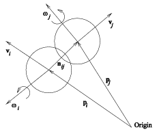
where is the force from pebble on pebble , is the force of the container on pebble , is the gravitational acceleration constant, is the mass of pebble , is the velocity of pebble , is the position vector for pebble , is the angular velocity of pebble i, is the tangential force between pebbles and , is the perpendicular force between pebbles and , is the radius of pebble , is the moment of inertia for pebble i, is the tangential force of the container on pebble i, is the unit vector normal to the container wall on pebble i, is the unit vector pointing from the position of pebble to that of pebble , is the current static friction loading between pebbles and , and is the function to compute the change in the static friction loading. The static friction model contributes to the term which is also part of the term. Figure 4.1 illustrates the principal vectors with pebble going in the direction and rotating around the axis, and pebble going in the direction and rotating around the axis.
The mass and moment of inertia are calculated assuming spherical symmetry with the equations:
| (4.5) |
| (4.6) |
where is the radius of inner (fueled) zone of the pebble, is the radius of whole pebble, is the average density of center fueled region and is the average density of outer non-fueled region.
The dynamic (or kinetic) friction model is based on the model described by Wait (2001). Wait’s and PEBBLES model calculate the dynamic friction using a combination of the relative velocities and pressure between the pebbles, as shown in Equations (4.7) and (4.8):
| (4.7) |
| (4.8) |
where is the tangential dash-pot constant, is the normal dash-pot constant, is the normal force between pebbles i and j, is the tangential dynamic friction force between pebbles i and j, is the normal Hooke’s law constant, is the overlap between pebbles i and j, is the component of the velocity between two pebbles perpendicular to the line joining their centers, is the component of the velocity between two pebbles parallel to the line joining their centers, is the relative velocity between pebbles i and j and is the kinetic friction coefficient. Equations (4.9-4.12) relate supplemental variables to the primary variables:
| (4.9) |
| (4.10) |
| (4.11) |
| (4.12) |
The friction force is then bounded by the friction coefficient and the normal force, to prevent it from being too great:
| (4.13) |
| (4.14) |
where is the static friction force between pebbles and , is the kinetic friction force between pebbles and , is the coefficient for force from slip, is the slip distance perpendicular to the normal force between pebbles and , is the maximum velocity under which static friction is allowed to operate, and is the static friction coefficient when the velocity is less than and the kinetic friction coefficient when the velocity is greater. These equations fully enforces the first requirement of a static friction method, .
When all the position, linear velocity, angular velocity and slips are combined into a vector , the whole computation can be written as a differential formulation in the form:
This can be solved by a variety of methods with the simplest being Euler’s method:
| (4.17) |
In addition, both the Runge-Kutta method and the Adams-Moulton method can be used for solving this equation. These methods improve the accuracy of the simulation. However, they do not improve the wall-clock time at the lowest stable simulation, since the additional time required for computation negates the advantage of being able to use somewhat longer time-steps. In addition, when running on a cluster, more data needs to be transferred since the methods allow non-contacting pebbles to affect each other in a single ‘time-step calculation’.
For any geometry interaction, two things need to be calculated, the overlap distance (or, technically, the mutual approach of distant points) and the normal to the surface . The input is the radius of the pebble and the position of the pebble, with components , , and
For the floor contact this is:
For cylinder contact on the inside of a cylinder this is:
For cylinder contact on the outside of a cylinder this is:
For contact on the inside of a cone defined by the :
These equations are derived from minimizing the distance between the contact point and the pebble position .
For contact on a plane defined by where the equation has been normalized so that , the following is used:
Combinatorial geometry operations can be done. Intersections and unions of multiple geometry types are done by calculating the overlaps and normals for all the geometry objects in the intersection or union. For an intersection, where there is overlap on all the geometry objects, then the smallest overlap and associated normal are kept, which may be no overlap. For a union, the largest overlap and its associated normal are kept.
For testing that a geometry is correct, a simple check is to fill up the geometry with pebbles using one of the methods described in Section 4.4, and then make sure that linear and angular energy dissipate. Many geometry errors will show up by artificially creating extra linear momentum. For example, if a plane is only defined at the top, but it is possible for pebbles to leak deep into the bottom of the plane, they will go from having no overlap to a very high overlap, which will give the pebble a large force. This results in extra energy being added each time a pebble encounters the poorly defined plane, which will show up in energy tallies.
The pebbles are packed using three main methods. The simplest creates a very loose packing with an approximately 0.15 packing fraction by randomly choosing locations, and removing the overlapping ones. These pebbles then allowed to fall down to compact to a realistic packing fraction.
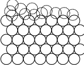
The second is the PRIMe method developed by Kloosterman and Ougouag (2005). In this method large numbers of random positions (on the order of 100,000 more than will fit) are generated. The random positions are sorted by height, and starting at the bottom, the ones that fit are kept. Figure 4.2 illustrates this process. This generates packing fractions of approximately 0.55. Then they are allowed to fall to compact. This compaction takes less time than starting with a 0.15 packing fraction.
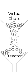
The last method is to automatically generates virtual chutes above the bed where the actual inlet chutes are, and then loads the pebbles into the chutes. Figure 4.3 shows this in progress. This allows locations that have piles where the inlet chutes are, but can be done quicker than a recirculation. The other two methods generate flat surfaces at the top, which is unrealistic, since the surface of a recirculated bed will have cones under each inlet chute.
The typical parameters used with the PEBBLES code are described in Table 4.1. Alternative numbers will be described when used.
|
The static friction model in PEBBLES is used to calculate the force and magnitude of the static friction force. Other models have been created before to calculate static friction, but the PEBBLES model provides the combination of being a differential model (as opposed to one where the force is rotated as a separate step) and being able to handle the type of geometries that exist in pebble bed reactors.
The static friction model has two key requirements. First, the force from stuck-slip must be updated based on relative motion of the pebbles. Second, the current direction of the force must be calculated since the pebbles can rotate in space.
For elastic spheres, the true method of updating the stuck-slip force is to use the method of Mindlin and Deresiewicz (1953). This method requires computationally and memory intensive calculations to track the forces. Instead, a simpler method is used to approximate the force. This method, described by Cundall and Strack (1979) uses the integration of the parallel relative velocity as the displacement. The essential idea is that the farther the pebbles have stuck-slipped at the contact point, the greater the counteracting static friction force needs to be. This is what happens under more accurate models such as Mindlin and Deresiewicz. There are two approximations imposed by this assumption. First, the amount the force changes is independent of the normal force. Second, the true hysteretic effects that are dependent on details of the loading history are ignored. For simulations where the exact dynamics of static friction are important, these could potentially be serious errors. However, since static friction only occurs when the relative speed is low, the dynamics of the simulation usually are unimportant. Thus, for most circumstances, the following approximation can be used for the rate of change of the magnitude and non-rotational change of the stuck-slip:
| (5.1) |
The slips can build up to unrealistically large amounts, that is, greater than ; equation 5.1 places no limit on the maximum size of the slip. The excessive slip is solved at two different locations. First, when the frictions are added together to determine the total friction they are limited by in equation (4.14). This by itself is insufficient, because the slip is storing potential energy that appears anytime the normal force increases. This manifests itself by causing vibration of the pebbles to continue for long periods of time. Two methods for fixing the hidden slip problem are available in PEBBLES. The simplest drops any slip that exceeds the static friction threshold (or an input parameter value somewhat above the static friction threshold so small vibrations do not cause the slip to disappear).
The second method used in PEBBLES is to decrease the slip that is over a threshold value. If the slip is too great, a derivative that is the opposite as the current slip is added as an additional term in the slip time derivative. This occurs in the following additional term:
| (5.2) |
In this is the ramp function (which is if and 0 otherwise), is a constant to select how much the slip is allowed to exceed the static friction threshold (usually 1.1 in PEBBLES). This derivative adder is used in most PEBBLES runs since it does allow vibrational energy to decrease, yet does not cause the pyramid benchmark to fail like complete removal of too great slips does.
When using non-Euler integration methods, the change in slip is calculated multiple times. Each time it is calculated, it might be set to be zeroed. In the PEBBLES code, if any of the added up slips for a given contact were set to be zeroed, the final slip is zeroed. This is not an ideal method, but it works well enough.
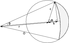
The static friction force must also be rotated so that it is in the plane of contact between the two pebbles. When there is a difference between the pebbles’ center velocities, which changes in the relative pebble center location, change in the direction in the stuck-slip occurs. That is:
| (5.3) |
First, let and . The cross product is perpendicular to both and and signed to create the axis around which is rotated in a right-handed direction. Then, using the cross product of the axis and , gives the correct direction that should be increased.
Next, determine the factors required to make the differential the proper length. By cross product laws,
| (5.4) |
where is the angle between and and is the angle between and .
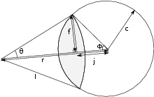
The relevant vectors are shown in figure 5.1.
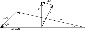
The goal is to rotate by angle which is the ‘projection’ into the proper plane of the angle that rotates by. Since the direction has been determined, for simplicity the figure leaves the indexes off, and concentrates on determining the lengths. In Figure 5.1, is the old slip vector, is the new slip vector, is the vector pointing from one pebble to another. The vector is added to to get the new , . The initial condition is that and are perpendicular. The final conditions are that and are perpendicular, and that and are the same length and that is the closest vector to as it can be while satisfying the other conditions. There is no requirement that or are coplanar with (otherwise would be equal to ). From the law of sines we have:
| (5.5) |
so
| (5.6) |
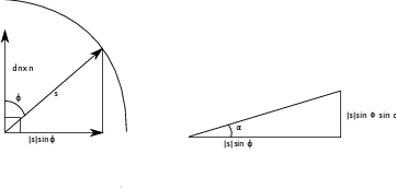
In Figure 5.2 the projection to the correct plane occurs. First by using the length of is projected to the plane. Note that is the angle both to and to . So, the length of the line on the plane is , and the length of the straight line at the end of the triangle is (note that the chord length is , but as approaches 0 the other can be used). From these calculations, the length of the can be calculated with the following formula:
| (5.7) |
Since the formula for the rotation is:
| (5.8) |
As a differential equation this is:
| (5.9) |
By the vector property and since , this can be rewritten as the version in Silbert et al. (2001):
| (5.10) |
It might seem that the wall interaction could be modeled the same way as the pebble-to-pebble interaction. For sufficiently simple wall geometries this may be possible, but actual pebble bed reactor geometries are more complicated, and violate some of the assumptions that underpin the derivation. For a flat surface, there is no rotation, so the formula can be entirely dropped. For a spherical surface, it would be possible to measure the curvature at pebble to surface contact point in the direction of relative velocity to the surface. This curvature could then be used as an effective radius in the pebble-to-pebble formulas.
The pebble reactor walls have additional features that violate assumptions made for the derivation. For surfaces such as a cone, the curvature is not in general constant, because the path can follow elliptical curves. As well, the curvature has discontinuities where different parts of the reactor join together (for example, the transition from the outlet cone to the outlet chute). At these transitions, the assumption that the slip stays parallel to the surface fails because the slip is parallel to the old surface, but the new surface has a different normal.
Because of the complications with using the pebble to pebble interaction, PEBBLES uses an approximation of the “rotation delta.” This is similar to the Vu-Quoc and Zhang (1999) method of adjusting the slip so that it is parallel to the surface each time. Each time when the slip is used, a temporary version of the slip that is properly aligned to the surface is computed and used for calculating the force. As well, a rotation to move the slip more parallel to the surface is also computed.
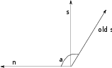
The rotation is computed as follows. Let the normal direction of the wall at the point of contact of the pebble be , and the old stuck-slip be . Let be the angle between and . is perpendicular to both and and so this cross product is the axis that needs to be rotated around. Then is perpendicular to this vector, so it is either pointing directly towards if is acute or directly away from if is obtuse. To obtain the correct direction, this vector is multiplied by the scalar which has the correct sign from . The magnitude of needs to be determined for reasonableness. We define the angle , which is between and . By these definitions the magnitude is . is a right angle since is perpendicular to , so . Collecting terms gives the magnitude as which is divided by to give the full term the magnitude . This is the length of the vector that goes from to the plane perpendicular to . This produces equation 5.11, which can be used to ensure that the wall stuck-slip vector rotates towards the correct direction.
| (5.11) |
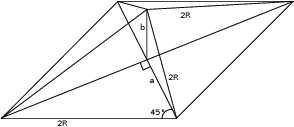
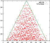
Static friction is an important physical feature in the implementation of mechanical models of pebbles motion in a pebble bed, and checking its correctness is important. A pyramid static friction test model was devised as a simple tool for verifying the implementation of a static friction model within the code. The main advantages of the pyramid test are that the model test is realistic and that it can be modeled analytically, providing an exact basis for the comparison. The test benchmark consists of a pyramid of five spheres on a flat surface. This configuration is used because the forces acting on each pebble can be calculated simply and the physical behavior of a model with only kinetic friction is fully predictable on physical and mathematical grounds: with only kinetic friction and no static friction, the pyramid will quickly flatten. Even insufficient static friction will result in the same outcome. The four bottom spheres are arranged as closely as possible in a square, and the fifth sphere is placed on top of them as shown in Fig. 5.4.
The lines connecting the centers of the spheres form a pyramid with sides , as shown in Fig. 5.5, where is the radius of the spheres. The length of in the figure is , and because is part of a right triangle, , so has the same length as , and thus the elevation angle for all vertexes of the pyramid are from horizontal.
Taking for origin of the coordinates system the projection of the pyramid summit onto the ground, the locations (coordinates) of the sphere centers are given in Table 5.1.
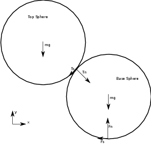
The initial forces on the base sphere are the force of gravity , and the normal forces and as shown in Fig. 5.6. This causes initial stuck-slip which will cause to develop to counter the slip, and to counter the rotation of the base sphere relative to the top sphere. The top sphere will have no rotation because the forces from the four spheres will be symmetric and counteract each other.
The forces on the base sphere are:
Note that is larger than since is only a portion of the force since the top sphere transmits (and splits) its force onto all four base spheres.
There are three requirements for a base sphere to be non-accelerated.
If a base sphere is not rotating than there is no torque, so:
| (5.12) |
The resultant of all forces must also be zero in the x and the y direction (vector notation dropped since they are in one dimension and therefore scalars) as follows:
| (5.13) |
| (5.14) |
Since the angle of contact between a base sphere and the top sphere is , the following two equations hold (where is the magnitude of and is the magnitude of ):
| (5.15) |
| (5.16) |
This changes equations 5.13 and 5.14 into:
| (5.17) |
| (5.18) |
Combining equation 5.12 and 5.17 provides:
| (5.19) |
Which gives the relation:
| (5.20) |
By the static friction Equation 3.1,
| (5.21) |
Combining equations 5.20 and 5.21 and simplifying gives the requirement that
| (5.22) |
For use with testing, the static friction program can be tested twice with a sphere-to-sphere friction coefficient slightly above 0.41421... and one slightly below 0.41421.... In the first case the pyramid should be stable, and in the second case the top ball should fall to the floor.
Since ¼ of the weight of the top pebble is on one of the base pebbles, the following holds:
| (5.23) |
Combining 5.18 and 5.23 provides the following equation:
| (5.24) |
Equations 5.17 and 5.24 can be added to produce
| (5.25) |
Using 5.12 and 5.24 and solving for Fs gives the following value for Fs:
| (5.26) |
By the static friction Equation 3.1:
| (5.27) |
Substituting the values for and gives:
| (5.28) |
Simplifying provides the following relation for the surface-to-sphere static friction requirement:
| (5.29) |
This can be used similarly to the other static friction requirement by setting the value slightly above 0.08284... and slightly below 0.08284... and making sure that it is stable with the higher value and not stable with the lower value.
This test was inspired by an observation of lead cannon balls stacked into a pyramid. I tried to stack used glass marbles into a five ball pyramid and it was not stable. Since lead has a static friction coefficient around 0.9 and used glass has a much lower static friction, the physics of pyramid stability was further investigated, resulting in this benchmark test of static friction modeling.
The benchmark test of two critical static friction coefficients is defined by the following equations. If both static friction coefficients are above the critical values, the spheres will form a stable pyramid. If either or both values are below the critical values the pyramid will collapse.
| (5.30) |
| (5.31) |
To set up the test cases, the sphere locations from Table 5.1 should be used as the initial locations of the sphere. Then, static friction coefficients for the sphere-to-sphere contact and the sphere-to-surface contact are chosen. The code is then run until either the center sphere falls to the surface, or the pyramid obtains a stable state. There are three test cases that are run to test the model.
For soft sphere models, there are fundamental limits to how close the model’s results can be to the critical coefficient. Essentially, as the critical coefficients are approached, the assumptions become less valid. For example, with soft (elastic) spheres, the force from the center sphere will distort the contact angle, so the actual critical value will be different. For the PEBBLES code, an value of 0.001 is used.
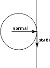
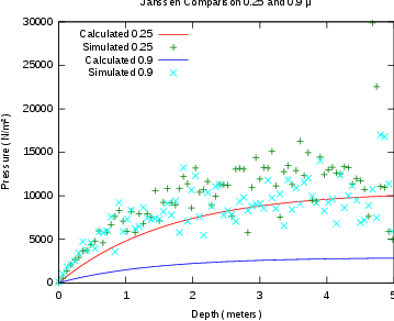
The pyramid static friction test is used as a simple test of the static friction model. Another test compares the static friction model against the Janssen formula’s behavior (Sperl, 2006). This formula specifies the expected wall pressure as a function of depth. This formula only applies when the static friction is fully loaded, that is when . This condition is generally not satisfied until some recirculation has occurred. Figure 5.7 shows the normal force and the static friction force from a pebble to the wall. With the PEBBLES code, this is only satisfied after recirculation with lower values of the static friction coefficient .
The equation used to calculate the pressure on the region from the normal force in PEBBLES is:
| (5.32) |
where is the pressure, is the height of the region, and is the radius of the cylinder.
The equation for calculating the Janssen formula pressure is
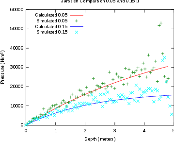
where is the pebble to pebble static friction coefficient, is the pebble to wall, is the packing fraction, is the density, is the gravitational acceleration, and is the depth that the pressure is being calculated. For the Figures 5.8 and 5.9, a packing fraction of 0.61 is used and a density of 1760 kg/m are used. There are 20,000 pebbles packed into a 0.5 meter radius cylinder, and 1,000 are recirculated before the pressure measurement is done.
Figure 5.8 compares the Janssen model with the PEBBLES simulation for static friction values of 0.05 and 0.15. For this case, the Janssen formula and the simulated pressures match closely. Figure 5.9 compares these again. In this case, the 0.25 values only approximately match, and the 0.9 static friction pressure values do not match at all. The static friction slip vectors were examined, and they are not perfectly vertical, and they are not fully loaded. This results in the static friction force being less than the maximum possible, and thus the pressure is higher since less of the force is removed by the walls.
Modeling the full physical effects that occur in a pebble bed reactor mechanics is not computationally possible with current computer resources. In fact, even modeling all the intermolecular forces that occur between two pebbles at sufficient levels to reproduce all macroscopic behavior is probably computationally intractable at the present time. This is partially caused by the complexity of effects such as inter-grain boundaries and small quantities of impurities that affect the physics and different levels between the atomic effects and the macroscopic world. Instead, all attempts at modeling the behavior of pebble bed reactor mechanics have relied on approximation to make the task computationally practical. The PEBBLES simulation has as high or higher fidelity than past efforts, but it does use multiple unphysical approximations. This chapter will discuss the approximations so that future simulation work can be improved, and an understanding of what limitations exist when applying PEBBLES to different problems.
In different regions of the reactor, the radioactivity and the fission will heat the pebbles differently, and the flow of the coolant helium will distribute this heat around the reactor. This will change the temperature of different parts of the reactor. Since the temperature will be different, the parameters driving the mechanics of the pebbles will be different as well. This includes parameters such as the static friction coefficients and the size of the pebbles which will change through thermal expansion. As well, parameters such as static friction can also vary depending on the gas in which they currently are in and in which they were, since some of the gas tends to remain in and on the carbon surface. Graphite dust produced by wear may also affect static friction in downstream portions of the reactor.
The pebbles in a pebble bed reactor have helium gas flowing around and past them. PEBBLES and all other pebble bed simulations ignore effects of this on pebble movement. However, the gas will cause both additional friction when the pebbles are dropping through the reactor, and the motion of gas will cause additional forces on pebbles.
Pebble bed mechanics simulations use soft spheres. Physically, there will be deflection of spheres under pressure (even the pressure of just one sphere on the floor), but the true compression is much smaller than what is actually modeled. In PEBBLES, the forces are chosen to keep the compression distance at a millimeter or below. Another effect related to the physics simulation is that force is transmitted via contact. This means the force from one end of the reactor is transmitted at a speed related to the time-step used for the simulation, instead of the speed of sound.
Since simulating billions of time-steps is time consuming, two approximations are made. First, instead of simulating the physical time that pebble bed reactors have between pebble additions (on the order of 2-5 minutes), new pebbles are added at a rate between a quarter second and two seconds. This may result in somewhat unphysical simulations since some vibration that would have dampened out with a longer time between pebble additions still exists when the next pebble impacts the bed. Second, since full recirculation of all the pebbles is computationally costly, for some simulations, only a partial recirculation or no recirculation is done.
The physics models do not take into account several physical phenomena. The physics do not handle pure spin effects, such as when two pebbles are contacting and are spinning with an axis around the contact point. This should result in forces on the pebbles, but the physics model does not handle this effect since the contact velocity is calculated as zero. In addition, when the pebble is rolling so that the contact velocity is zero because the pebble’s turning axis is parallel to the surface and at the same rate as the pebble is moving along the surface, there should be rolling friction, but this effect is not modeled either. As well, the equations used assume that the pebbles are spherically symmetric, but defects in manufacturing and slight asymmetries in the TRISO particle distribution mean that there will be small deviations from being truly spherically symmetric.
The physics model does not match classical Hertzian or Mindlin and Deresiewicz elastic sphere behavior. The static friction model is a simplification and does not capture all the hysteretic effects of true static friction. Effectively, this means that , the coefficient used to calculate the force from slip, is not a constant. In order to fully discuss this, some features of these models will be discussed in the following paragraphs.
Since closed-form expressions exist for elastic contact between spheres, they will be used, instead of a more general case which lacks closed-form expressions. Spheres are not a perfect representation of the effect of contact between shapes such as a cone and a sphere, but should give an approximation of the size of the effect of curvature.
The amount of contact area and displacement of distant points for two spheres or one sphere and one spherical hole (that is negative curvature) for elastic spheres can be calculated via Hertzian theory(Johnson, 1985). For two spherical surfaces the following variables are defined:
| (6.1) |
and
| (6.2) |
with the th’s sphere’s radius, the Young’s modulus, the Poisson’s ration of the material. For a concave sphere, the radius will be negative. Then, via Hertzian theory, the contact circle radius will be:
| (6.3) |
where is the normal force. The mutual approach of distant points is given by:
| (6.4) |
Notice that the above differs compared to the Hooke’s Law formulation that PEBBLES uses. The maximum pressure will be:
| (6.5) |
So as a function of the radii and , the circle radius of the contact will be:
| (6.6) |
If is used for the multiple of negative curvature sphere of the radius of the other, then the equation becomes:
| (6.7) |
which can be rearranged to:
| (6.8) |
From this equation, as increases, it has less effect on contact area, so if is much greater than , the contact area will tend to be dominated by rather than . For example, typical radii in PEBBLES might be 18 cm outlet chute and a 3 cm pebble, which would put at 6, so the effect on contact area radius would be about 33% difference compared to pebble to pebble contact area radius, or 6% compared to a flat surface.1
To some extent, the actual contact area is irrelevant for calculating the maximum static friction force as long as some conditions are met. Both surfaces need to be of a uniform material. The basic macroscopic description needs to hold, so changing the area changes the pressure , but not the maximum static friction force. If the smaller area causes the pressure to increase enough to cause plastic rather than elastic contact, then through that mechanism, the contact area would cause actual differences in experimental values. PEBBLES also does not calculate plastic contact effects.
The contact area causes an effect through another mechanism. The tangential compliance in the case of constant normal and increasing tangential force, that is the slope of the curve relating displacement to tangential force, is given in Mindlin and Deresiewicz as:
| (6.9) |
Since the contact area radius, , is a function of curvature, the slope of the tangential compliance will be as well, which is another effect that PEBBLES’ constant does not capture.
In summary for the static friction using a constant coefficient for yields two different approximations. First, using the same constants for wall contact when there is different curvatures is an approximation that will give somewhat inconsistent results. Since the equations for spherical contact are dominated by the smaller radius object, this effect is somewhat less but still exists. Second, using the same constant coefficient for different loading histories is a approximation. For a higher fidelity, these effects need to be taken into account.
Planned and existing pebble bed reactors can have on the order of 100,000 pebbles. For some simulations, these pebbles need to be followed for long time periods, which can require computing billions of time-steps. Multiplying the time-steps required by the number of pebbles being computed over leads to the conclusion that large numbers of computations are required. These computations should be as fast as possible, and should be as parallel as possible, so as to allow relevant calculations to be done in a reasonable amount of time. This chapter discusses the process of speeding up the code and parallelizing it.
The PEBBLES program has three major portions of calculation. The first is determining which pebbles are in contact with other pebbles. The second computational part is determining the time derivatives for all the vectors for all the pebbles. The third computational part is using the derivatives to update the values. Overall, for calculation of a single time-step, the algorithm’s computation time is linearly proportional to the number of pebbles, that is O(n)1 .
There are four different generic parts of the complete calculation that need to considered for determining the overall speed. The first consideration is the time to compute arithmetic operations. Modern processors can complete arithmetic operations in nanoseconds or fractions of nanoseconds. In the PEBBLES code, the amount of time spent on arithmetic is practically undetectable in wall clock changes. The second consideration is the time required for reading memory and writing memory. For main memory accesses, this takes hundreds of CPU clock cycles, so these times are on the order of fractions of microseconds (Drepper, 2007). Because of the time required to access main memory, all modern CPUs have on-chip caches, that contain a copy of the recently used data. If the memory access is in the CPU’s cache, the data can be retrieved and written in a small number of CPU cycles. Main memory writes are somewhat more expensive than main memory reads, since any copies of the memory that exist in other processor’s caches need to be updated or invalidated. So for a typical calculation like the time spent doing the arithmetic is trivial compared to the time spent reading in and and writing out .
The third consideration is the amount of time required for parallel programming constructs. Various parallel synchronization tools such as atomic operations, locks and critical sections take time. These take an amount of time on the same order of magnitude as memory writes. However, they typically need a read and then a write without any other processor being able to access that chunk of memory in between which requires additional overhead, and a possible wait if the memory address is being used by another process. Atomic operations on x86_64 architectures are faster than using locks, and locks are generally faster than using critical sections. The fourth consideration is network time. Sending and receiving a value can easily take over a millisecond for the round trip time. These four time consuming operations need to be considered when choosing algorithms and methods of calculation.
There are a variety of methods for profiling the computer code. The simplest method is to use the FORTRAN 95 intrinsics CPU_TIME and DATE_AND_TIME. The CPU_TIME subroutine returns a real number of seconds of CPU time. The DATE_AND_TIME subroutine returns the current wall clock time in the VALUES argument. With gfortran both these times are accurate to at least a millisecond. The difference between two different calls of these functions provide information on both the wall clock time and the CPU time between the calls. (For the DATE_AND_TIME subroutine, it is easiest if the days, hours, minutes, seconds and milliseconds are converted to a real seconds past some arbitrary time.) The time methods provide basic information and a good starting point for determining which parts of the program are consuming time. For more detailed profiling the oprofile (opr, 2009) program can be used on Linux. This program can provide data at the assembly language level which makes it possible to determine which part of a complex function is consuming the time. Non-assembly language profilers are difficult to accurately use on optimized code, and profiling non-optimized code is misrepresentative.
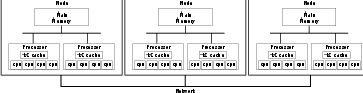
Parallel computers can be arranged in a variety of ways. Because of the expense of linking shared memory to all processors, a common architecture is a cluster of nodes with each node having multiple processors. Each node is linked to other nodes via a fast network connection. The processors on a single node share memory. Figure 7.1 shows this arrangement. For this arrangement, the code can use both the OpenMP (Open Multi-Processing) (ope, 2008) and the MPI (Message Passing Interface) (mpi, 2009) libraries. MPI is a programming interface for transferring data across a network to other nodes. OpenMP is a shared memory programming interface. By using both programming interfaces high speed shared memory accesses can be used on memory shared on the node and the code can be parallelized across multiple nodes.
For any granular material simulation, which particles are in contact must be determined quickly and accurately for each time-step. This is called collision detection, though for pebble simulations it might be more accurately labeled contact detection. The simplest algorithm for collision detection is to iterate over all the other objects and compare each one to the current object for collision. To determine all the collisions using that method, time is required.
An improved algorithm by Cohen et al. (1995) uses six sorted lists of the lower and upper bounds for each object. (There is one upper bound list and one lower bound list for each dimension.) With this algorithm, to determine the collisions for a given object, the bounds of the current objects are compared to bounds in the list—only objects that overlap the bounds in all three dimensions will potentially collide. This algorithm typically has approximately time,2 because of the sorting of the bounding lists (Cohen et al., 1995).
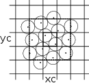
A third, faster method, grid collision detection, is available if the following requirements hold: (1) there is a maximum diameter of object, and no object exceeds this diameter, and (2) for a given volume, there is a reasonably small, finite, maximum number of objects that could ever be in that volume. These two constraints are easily satisfied by pebble bed simulations, since the pebbles are effectively the same size (small changes in diameter occur due to wear and thermal effects). A three-dimensional parallelepiped grid is used over the entire range in which the pebbles are simulated. The grid spacing is set at the maximum diameter of any object (twice the maximum radius for spheres).
Two key variables are initialized, , the number of pebbles in grid locations x,y,z; and , the pebble identification numbers () for each x,y,z location. The is a unique number assigned to each pebble in the simulation. The spacing between successive grid indexes is , so the index of a given x location can be determined by where is the zero x index’s floor; similar formulas are used for y and z.
The grid is initialized by setting , and then the x,y,z indexes are determined for each pebble. The at that location is then atomically3 incremented by one and fetched. Because OpenMP 3.0 does not have a atomic add-and-fetch, the lock xadd x86_64 assembly language instruction is put in a function. The provides the fourth index into the array, so the pebble can be stored into the array. The amount of time to zero the array is a function of the volume of space, which is proportional to the number of pebbles. The initialization iteration over the pebbles can be done in parallel because of the use of an atomic add-and-fetch function. Updating the grid iterates over the entire list of pebbles so the full algorithm for updating the grid is for the number of pebbles.
Once the grid is updated, the nearby pebbles can be quickly determined. Figure 7.2 illustrates the general process. First, index values are computed from the pebble and used to generate , , and . This finds the center grid location, which is shown as the bold box in the figure. Then, all the possible pebble collisions must have grid locations (that is, their centers are in the grid locations) in the dashed box, which can be found by iterating over the grid locations from to and repeating for the other two dimensions. There are grid locations to check, and the number of pebbles in them are bounded (maximum 8), so the time to do this is bounded. Since this search does not change any grid values, it can be done in parallel without any locks.
Therefore, because of the unique features of pebble bed pebbles simulation, a parallel lock-less algorithm for determining the pebbles in contact can be created.
The PEBBLES code uses MPI to distribute the computational work across different nodes. The MPI/OpenMP hybrid parallelization splits the calculation of the derivatives and the new variables geometrically and passes the data at the geometry boundaries between nodes using messages. Each pebble has a primary node and may also have various boundary nodes. The pebble-primary-node is responsible for updating the pebble position, velocity, angular velocity, and slips. The pebble-primary-node also sends data about the pebble to any nodes that are the pebble boundary nodes and will transfer the pebble to a different node if the pebble crosses the geometric boundary of the node. Boundary pebbles are those close enough to a boundary that their data needs to be present in multiple nodes so that the node’s primary pebbles can be properly updated. Node 0 is the master node and does processing that is simplest to do on one node, such as writing restart data to disk and initializing the pebble data. The following steps are used for initializing the nodes and then transferring data between them:
Order of calculation and data transfers in main loop:
All the information and subroutines needed to calculate the primary and boundary nodes that a pebble belongs to are calculated and stored in a FORTRAN 95 module named network_domain_module. The module uses two derived types: network_domain_type and network_domain_location_type. Both types have no public components so the implementation of the domain calculation and the location information can be changed without changing anything but the module, and the internals of the module can be changed without changing the rest of the PEBBLES code. The location type stores the primary node and the boundary nodes of a pebble. The module contains subroutines for determining the location type of a pebble based on its position, primary and boundary nodes for a location type, and subroutines for initialization, load balancing, and transferring of domain information over the network.
The current method of dividing the nodes into geometric domains uses a list of boundaries between the z (axial) locations. This list is searched via binary search to find the nodes nearest to the pebble position, as well as those within the boundary layer distance above and below the zone interface in order to identify all the boundary nodes that participate in data transfers. The location type resulting from this is cached on a fine grid, and the cached value is returned when the location type data is needed. The module contains a subroutine that takes a work parameter (typically, the computation time of each of the nodes) and can redistribute the z boundaries up or down to shift work towards nodes that are taking less time computing their share of information. If needed in the future, the z-only method of dividing the geometry could be replaced with a full 3-D version by modifying the network domain module.
The PEBBLES code uses OpenMP to distribute the calculation over multiple processes on a single node. OpenMP allows directives to be given to the compiler that direct how portions of code are to be parallelized. This allows a single piece of code to be used for both the single processor version and the OpenMP version. The PEBBLES parallelization typically uses OpenMP directives to cause loops that iterate over all the pebbles to be run in parallel.
Some details need to be taken into consideration for the parallelization of the calculation of acceleration and torque. The physical accelerations imposed by the wall are treated in parallel, and there is no problem with writing over the data because each processor is assigned a portion of the total zone inventory of pebbles. For calculating the pebble-to-pebble forces, each processor is assigned a fraction of the pebbles, but there is a possibility of the force addition computation overwriting another calculation because the forces on a pair of pebbles are calculated and then the calculated force is added to the force on each pebble. In this case, it is possible for one processor to read the current force from memory and add the new force from the pebble pair while another processor is reading the current force from memory and adding its new force to that value; they could both then write back the values they have computed. This would be incorrect because each calculation has only added one of the new pebble pair forces. Instead, PEBBLES uses an OpenMP ATOMIC directive to force the addition to be performed atomically, thereby guaranteeing that the addition uses the latest value of the force sum and saves it before a different processor has a chance to read it.
For calculating the sum of the derivatives using Euler’s method, updating concurrently poses no problem because each individual pebble has derivatives calculated. The data structure for storing the pebble-to-pebble slips (sums of forces used to calculate static friction) is similar to the data structure used for the collision detection grid. A 2-D array exists where one index is the from-pebble and the other index is for storing of the pebbles that have slip with the first pebble. A second array exists that contains the number of stored, and that number is always added and fetched atomically, which allows the slip data to be updated by multiple processors at once. These combine to allow the program to run efficiently on shared memory architectures.
The parallelization of the algorithm is checked by running the test case with a short number of time steps (10 to 100). Various summary data are checked to make sure that they match the values computed with the single processor version and between different numbers of nodes and processors. For example, with the NGNP-600 model used in the results section, the average overlap of pebbles at the start of the run is 9.665281e-5 meters. The single processor average overlap at the end of the 100 time-step run is 9.693057e-5 meters, the 2 nodes average overlap is 9.693043e-5 meters, and the 12 node average overlap is 9.693029e-5 meters. The lower order numbers change from run to run. The start-of-run values match each other exactly, and the end-of-run values match the start of run values to two significant figures. However, the three different end-of-run values match to five significant digits. In short, the end values match each other more than they match the start values. The overlap is very sensitive to small changes in the calculation because it is a function of the difference between two positions. During coding, multiple defects were found and corrected by checking that the overlaps matched closely enough between the single processor calculation and the multiple processor calculations. The total energy or the linear energy or other computations can be used similarly since the lower significant digits also change frequently and are computed over all the pebbles.
The data in Table 7.1 and Table 7.2 provide information on the time used with the current version of PEBBLES for running 80 simulation time steps on two models. The NGNP-600 model has 480,000 pebbles. The AVR model contains 100,000 pebbles. All times are reported in units of wall-clock seconds. The single processor NGNP-600 model took 251 seconds and the AVR single processor model took 48 seconds when running the current version. The timing runs were carried out on a cluster with two Intel Xeon X5355 2.66 GHz processors per node with a DDR 4X InfiniBand interconnect network. The nodes had 8 processors per node. The gfortran 4.3 compiler was used.
|
|
Significant speedups have resulted with both the OpenMP and MPI/OpenMP versions. A basic time step for the NGNP-600 model went from 3.138 seconds to 146 milliseconds when running on 64 processors. Since a full recirculation would take on the order of 1.6e9 time steps, the wall clock time for running a full recirculation simulation has gone from about 160 years to a little over 7 years. For smaller simulation tasks, such as simulating the motion of the pebbles in a pebble bed reactor during an earthquake, the times are more reasonable, taking about 5e5 time steps. Thus, for the NGNP-600 model, a full earthquake can be simulated in about 20 hours when using 64 processors. For the smaller AVR model, the basic time step takes about 34 milliseconds when using 64 processors. Since there are less pebbles to recirculate, a full recirculation would take on the order of 2.5e8 time steps, or about 98 days of wall clock time.
The knowledge of the packing and flow patterns (and to a much lesser extent the position) of pebbles in the pebble bed reactor is an essential prerequisite for many in-core fuel cycle design activities as well as for safety assessment studies. Three applications have been done with the PEBBLES code. The major application is the computation of pebble positions during a simulated earthquake. Two other applications that have been done are calculation of space dependent Dancoff factors and calculation of the angle of repose for a HTR-10 simulation.
|
|
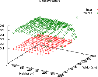
The calculation of Dancoff factors is an example application that needs accurate pebble position data. The Dancoff factor is used for adjusting the resonance escape probability for neutrons. There are two Dancoff factors that use pebble position data. The first is the inter-pebble Dancoff factor that is the probability that a neutron escaping from the fuel zone of a pebble crosses a fuel particle in another pebble. The second is the pebble-pebble Dancoff factor, which is the probability that a neutron escaping one fuel zone will enter another fuel zone without interacting with a moderator nuclide. Kloosterman and Ougouag (2005) use pebble location information to calculate the probability by ray tracing from fuel lumps until another is hit or the ray escapes the reactor. The PEBBLES code has been used for providing position information to J. L. Kloosterman and A. M. Ougouag’s PEBDAN program. This program calculate these factors as shown in Figure 8.2 which calculates them for the AVR reactor model.
The PEBBLES code was used for calculating the angle of repose for an analysis of the HTR-10 first criticality (Terry et al., 2006). The pebble bed code recirculated pebbles to determine the angle at which the pebbles would stack at the top of the reactor as shown in Figure 8.3, since this information was not provided, but was needed for the simulation of the reactor(Bäumer et al., 1990).
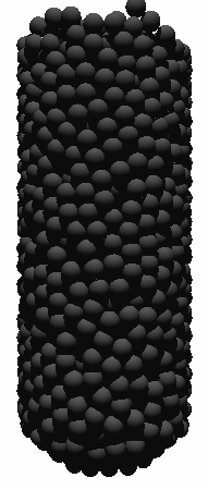
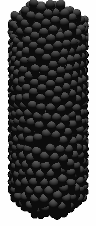
During experimental work before the construction of the AVR, it was discovered that when the pebbles were recirculated, the ordering in the pebbles increased. Figures 8.4 and 8.5 show that this effect occurs in the PEBBLES simulation as well. The final AVR design incorporated indentations in the wall to prevent this from occurring.
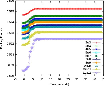
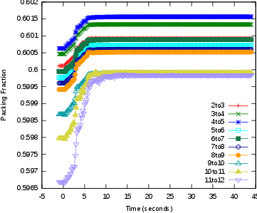
The packing fraction of the pebbles in a pebble bed reactor can vary depending on the method of packing and the subsequent history of the packing. This packing fraction can affect the neutronics behavior of the reactor, since it translates into an effective fuel density. During normal operation, the packing fraction will vary only slowly, over the course of weeks and then stabilize. During an earthquake, the packing fraction can increase suddenly. This packing fraction change is a concern since packing fraction increase can increase the neutron multiplication and cause criticality concerns as shown by Ougouag and Terry (2001).
The PEBBLES code can simulate this increase and determine the rate of change and the expected final packing fraction, thus allowing the effect of an earthquake to be simulated.
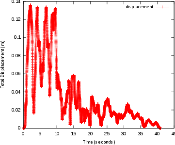
The movement of earthquakes has been well studied in the past. The magnitude of the motion of earthquakes is described by the Mercalli scale, which describes the maximum acceleration that a given earthquake will impart to structures. For a Mercalli X earthquake, the maximum acceleration is about 1 g. The more familiar Richter scale measures the total energy release of an earthquake (Lamarsh, 1983), which is not useful for determining the effect on a pebble bed core. For a given location, the soil properties can be measured, and using soil data and the motion that the bedrock will undergo, the motion on the surface can be simulated. The INL site had this information generated in order to determine the motion from the worst earthquake that could be expected over a 10,000 years period (Payne, 2003). This earthquake has roughly a Mercalli IX intensity. The data for such a 10,000 year earthquake are used for the simulation in this dissertation.
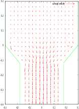
The code simulates earthquakes by adding a displacement to the walls of the reactor. As well, the velocity of the walls needs to be calculated. The displacement in the simulation can be specified either as the sum of sine waves, or as a table of displacements that specifies the x, y, and z displacements for each time. At each time step both the displacement and the velocity of the displacement are calculated. When the displacement is calculated by a sum of sine functions, the current displacement is calculated by adding vector direction for each wave and the velocity is calculated from the sum of the first derivative of all the waves. When the displacement is calculated from a table of data, the current displacement is a linear interpolation of the two nearest data points in the table, and the velocity is the slope between them. The walls are then assigned the appropriate computed displacement and velocity. Figure 8.6 shows the total displacement for the INL earthquake simulation specifications that were used in this paper.
The results of two simulations carried out here show a substantially safer behavior than the Ougouag and Terry (2001) bounding calculations. The methodology was applied to a model of the PBMR-400 model and two different static friction coefficients were tested, 0.65 and 0.35. The packing fraction increased from 0.593 to 0.594 over the course of the earthquake with the 0.65 static friction model, with the fastest increase was from 0.59307 to 0.59356 and took place over 0.8 seconds. With the 0.35 static friction model, the overall increase was from 0.599 to 0.601. The fasted increase was from 0.59964 to 0.60011 in 0.8 seconds. This is remarkably small when compared to the bounding calculation packing fraction increase rate of 0.129 sec in free fall.1 Both computed increases and packing fraction change rates are substantially below the free fall bounding rate and packing fraction change of a transition from 0.60 to 0.64 in 0.31 seconds. The computed rate and the total packing fraction increase are in the range that can be offset by thermal feedback effects for uranium fueled reactors.
During the course of the earthquake, the boundary density fluctuations (that is the oscillations in packing fraction near a boundary) are observed to increase in amplitude. Figure 8.9 shows the packing fraction before the earthquake and after the earthquake in the radial direction. These were taken from 4 to 8 meters above the fuel outlet chute in the PBMR-400 model. All the radial locations have increased packing compared to the packing fraction before the earthquake, but the points that are at boundary density fluctuation peaks increase the most. This effect can be seen in figure 8.10, which shows the increase in packing fraction before the earthquake and after
A previous version of the positional data from the earthquake simulation was provided to J. Ortensi. This data was used by him to simulate the effects of an earthquake on a pebble bed reactor(Ortensi, 2009). Essentially, two factors cause an increase in reactivity. The first is the increased density of the pebbles and the second is due to the control rods being at the top of reactor, so when the top pebbles move down the control rod worth (effect) decreases. However, the reactivity increase causes the fuel temperature to rise, which causes Doppler broadening and more neutrons are absorbed by the U, which causes the reactivity to fall. Figure 8.11 shows an example of this.
For each time-step, the simulation calculates both a displacement and a wall velocity.
For the sum of waves method, the displacement is calculated by:
| (8.1) |
where is the current time, is the time the wave starts, is the period of the wave, is the initial cycle of the wave, is the offset, and is the maximum displacement vector.
The velocity is calculated by:
| (8.2) |
For the tabular data, the displacement and velocity are calculated by:
where is the displacement at the th time-step, is a number between 0 and 1 that specifies where 0 is the start of the time-step and 1 is the end, and is the time in seconds between time-steps.
With these displacements, the code then uses:
as the adjusted position and velocity.
With the creation of the PEBBLES simulation, one issue that was examined was using the simulation to attempt to predict the volume of dust that would be produced by an operating pebble bed reactor. This is an important issue that could affect the choice of a pebble bed reactor versus a prismatic reactor for process heat applications. However, as this chapter and Appendix B will discuss, while the PEBBLES code has the force and motion data required for this simulation, the coefficients that would allow this information to be used have not been sufficiently robustly experimentally determined yet.
With the data provided by PEBBLES, equations to link the dust production to PEBBLES calculated quantities were examined. As shown in equation B.1, the volume of dust produced can be approximated if the normal force of contact, the length slide and the wear coefficients are known. The force of contact and the length slide are calculated as part of the PEBBLES simulation, so this method was used to calculate dust production for the AVR reactor. This resulted in an estimate of four grams of graphite dust produced per year as compared to the measured value of three kilograms of dust produced per year. Several possible causes of this were identified in the paper documenting this work (Cogliati and Ougouag, 2008). A key first issue as described by this dissertation’s previous work section is that there are no good measurements of graphite wear rates in pebble bed reactor relevant conditions (especially for a reactor run at AVR temperatures). A second issue is that the previous model of AVR was missing features including the reactor control rod nose cones and wall indentations. A third issue, identified after the paper’s publication, is that significant portions of the length traveled were due not to motion down through the reactor. Instead, much of the length that was tallied was due to pebbles vibrating. In the model used in the paper, this problem was about four times more severe than the current model, due to the new addition of slip correction via equation 5.2.
As an illustration of the general framework for dust production, a simple cylindrical vat the size of AVR was simulated. In this model, the outlet chute starts shrinking at height zero. The length (L), and length times normal force (NL) were tallied on intervals of 6 cm and the figures 9.1 to 9.5 show the results after recirculating 400 pebbles. The results are on a per pebble-pass basis. Two sets of static friction and kinetic friction pairs are used, one with a static friction coefficient of 0.35 and kinetic of 0.25, and the other with static of 0.65 and kinetic of 0.4. Figure 9.1 shows the calculated pebble-to-pebble lengths. Notice that for the 0.65 static friction simulation, about 10 meters of length traveled is occurring at the peak in a 6 cm long tally. Since the pebble is traveling about 0.06 m and has at most 12 pebble to pebble contacts, essentially all but a small portion of this length traveled is due to when the pebbles vibrate relative to each other. This vibration is caused by the impact of the pebbles coming from the inlet chutes and hitting the top of the bed. This likely is a true physical effect, which has not been discussed in literature this author is aware of. However, in order to obtain the correct magnitude of this vibrational effect, two things must be correct. First, the simulation must dissipate the vibration at the correct rate, and second, the pebbles must impact the bed at the correct velocity. Quality estimates of both will need to be made to finish the dust production work. Note that with the lower static friction value, the effect is even more pronounced.
Figure 9.2 is also expected to have a vibrational component, since only a small portion of pebbles should contact the wall, and therefore for a 6 cm tally, the length traveled by the average pebble should be much lower than 6 cm. As the chute is entered, the distance the average pebble travels increases in the 0.65 static friction case. Figure 9.3 shows the average normal contact force. The peak value for the pebble to surface values is due to the base of the ‘arch’ formed by pebbles. The curves for both the 0.65 static friction coefficient and the 0.35 static friction coefficient are approximately the same because the static friction force is not reaching the full Coulomb limit, so both have the same effective .
Figure 9.4 shows the normal times force sums. For the 0.65 case, the peak is due to the vibrational impact. For the 0.35 case, the vibration travels deep into the reactor bed, producing dust throughout the reactor. Figure 9.5 shows the peak dust production coming in the base of the reactor, where the forces are the highest, and the greatest lengths are traveled next to the wall.
The dust production simulation requires both proper dust production wear coefficients, and properly determining the correct method of dealing with vibrational issues. It would be useful to determine the number of pebbles that need to be simulated to provide a correct representation of a full NGNP-600 sized reactor. Since the middle portions are geometrically similar, determining the amount of recirculation that is required to reach a geometrically asymptotic state might allow only a portion of the recirculation to be done. Those two changes might allow quicker simulation of full sized reactors. Finally, in order to allow sufficiently fast simulations on today’s computer hardware many approximations to the true behavior are done. In the future, some of these approximations maybe relaxed.
Research results presented in this dissertation demonstrates a distinct element method that provides high fidelity and yet has reasonable run-times for many pebble fuel element flow simulations. The new static friction test will be useful for evaluating any implementation of static friction for spheres. The PEBBLES code produced for this dissertation has been able to provide data for multiple applications including Dancoff factor calculation, neutronics simulation and earthquake simulation. The new static friction model provides expected static friction behavior in the reactor including partial matching of the Janssen model predictions and correctly matching stability behavior in a pyramid. The groundwork has been created for predicting the dust production from wear in a pebble bed reactor once further experimental data is available. Future work includes potentially relaxing some of the physical approximations made for speed purposes when faster computing hardware exists, and investigating new methods for allowing faster simulations. This dissertation has provided significant enhancements in simulation of the mechanical movement of pebbles in a pebble bed reactor.
Mpi: A message-passing interface standard, version 2.2. 2009. URL http://www.mpi-forum.org/docs/mpi-2.2/mpi22-report.pdf.
Openmp application program interface, version 3.0. 2008. URL http://www.openmp.org/mp-documents/spec30.pdf.
Oprofile - a system profiler for linux. 2009. URL http://oprofile.sourceforge.net.
The commissioning of the thtr 300. a performance report, a. D HRB 129288E.
Hkg hochtemperatur-kernkraftwerk gesellschaft mit beschränkter haftung, b. http://www.thtr.de/ Accessed Oct 27, 2009. Technical data on: http://www.thtr.de/technik-tht.htm.
Atomwirtschaft-Atomtechnik-atw. Avr-atomversuchskraftwerk mit kugelhaufen-hochtemperatur-reaktor in juelich. Atomwirtschaft, May 1966. Sonderdruck aus Heft (Available as part of NEA-1739: IRPhE/AVR http://www.nea.fr/abs/html/nea-1739.html. Pages particularly useful are 230 and 240).
R. Bäumer, H. Barnert, E. Baust, A. Bergerfurth, H. Bonnenberg, H. Bülling, St. Burger, C.-B. von der Decken, W. Delle, H. Gerwin, K.-G. Hackstein, H.-J. Hantke, H. Hohn, G. Ivens, N. Kirch, A. I. Kirjushin, W. Kröger, K. Krüger, N. G. Kuzavkov, G. Lange, C. Marnet, H. Nickel, P. Pohl, W. Scherer, J. Schöning, R. Schulten, J. Singh, W. Steinwarz, W. Theymann, E. Wahlen, U. Wawrzik, I. Weisbrodt, H. Werner, M. Wimmers, and E. Ziermann. AVR: Experimental High Temperature Reactor; 21 years of sucessful operation for a future energy technology. Association of German Engineers (VDI), The Society for Energy Technologies, 1990. ISBN 3-18-401015-5.
D. Bedenig, W. Rausch, and G. Schmidt. Parameter studies concerning the flow behaviour of a pebble with reference to the fuel element movement in the core of the thtr 300 mwe prototype reactor. Nuclear Engineering and Design, 7:367–378, 1968.
R.F. Benenati and C. B. Brosilow. Void fraction distribution in beds of spheres. A. I. Ch. E. Journal, 8:359–361, 1962.
J. D. Bernal, J. Mason, and G. David Scott. Packing of spheres. Nature, 188:908–911, 1960.
Bharat Bhushan. Modern Tribology Handbook. CRC Press, Boca Raton, Florida, USA, 2000. Chap. 7.5.
I. Bratberg, K.J. Maløy, and A. Hansen. Validity of the janssen law in narrow granular columns. The European Physical Journal E, 18:245–252, 2005.
J. J. Cogliati and A. M. Ougouag. Pebble bed reactor dust production model. Proceedings of the 4th International Topical Meeting on High Temperature Reactor Technology, 2008. Washington, D.C., USA, September 28 – October 1.
Jonathan D. Cohen, Ming C. Lin, Dinesh Manocha, and Madhav K. Ponamgi. Icollide: an interactive and exact collision detection system for large scale environments. Proceedings of the 1995 Symposium on Interactive 3D Graphics, 1995. Monterey, CA, April 9-12, pp. 19-24.
P. A. Cundall and O. D. L. Strack. A discrete numerical model for granular assemblies. Géotechniqe, 29:47–65, 1979.
Ulrich Drepper. What every programmer should know about memory. 2007. URL http://people.redhat.com/drepper/cpumemory.pdf.
Jacques Duran. Sands, Powders, and Grains: An Introduction to the Physics of Granular Materials. Springer, New York, New York, USA, 1999. ISBN 978-0387986562.
Hannsjörg Freund, Thomas Zeiser, Florian Huber, Elias Klemm, Gunther Brenner, Franz Durst, and Gerhand Emig. Numerical simulations of single phase reacting flows in randomly packed fixed-bed reactors and experimental validation. Chemical Engineering Science, 58:903–910, 2003.
A. J. Goodjohn. Summary of gas-cooled reactor programs. Energy, 16: 79–106, 1991.
Keishi Gotoh, Hiroaki Masuda, and Ko Higashitanti. Powder Technology Handbook, 2nd ed. Marcel Dekker, Inc, New York, New York, 1997.
Hans D. Gougar, Abderrafi M. Ougouag, and William K. Terry. Advanced core design and fuel management for pebble-bed reactors. 2004. INEEL/EXT-04-02245.
J. M. Haile. Molecular Dynamics Simulation. John Wiley & Sons, Inc, New York, 1997.
K.L. Johnson. Contact Mechanics. Cambridge University Press, 1985. ISBN 0-521-34796-3. Section 4.2.
Rémi Jullien, André Pavlovitch, and Paul Meakin. Random packings of spheres built with sequential models. Journal Phys. A: Math. Gen., 25: 4103–4113, 1992.
Andrew C. Kadak and Martin Z. Bazant. Pebble flow experiments for pebble bed reactors. Bejing, China, September 22-24 2004. 2nd International Topical Meeting on High Temperature Reactor Technology.
J. L. Kloosterman and A. M. Ougouag. Computation of dancoff factors for fuel elements incorporating randomly packed triso particles. Technical report, 2005. INEEL/EXT-05-02593, Idaho National Laboratory.
G. A. Kohring. Studies of diffusional mixing in rotating drums via computer simulations. Journal de Physique I, 5:1551, 1995.
J.R. Lamarsh. Introduction to Nuclear Engineering 2nd Ed. Addison-Wesley Publishing Company, Reading, Massaschusetts, 1983. pp. 591-593.
J.K. Lancaster and J.R. Pritchard. On the ‘dusting’ wear regime of graphite sliding against carbon. J. Phys. D: Appl. Phys., 13:1551–1564, 1980.
James W. Landry, Gary S. Grest, Leonardo E. Silbert, and Steven J. Plimpton. Confined granular packings: Structure, stress, and forces. Physical Review E, 67:041303, 2003.
Zi Lu, Mohamed Abdou, and Alice Ying. 3d micromechanical modeling of packed beds. Journal of Nuclear Materials, 299:101–110, 2001.
Xiaowei Luo, Lihong Zhang, and Yu Suyuan. The wear properties of nuclear grade graphite ig-11 under different loads. International Journal of Nuclear Energy Science and Technology, 1(1):33–43, 2004.
Xiaowei Luo, Yu Suyuan, Sheng Xuanyu, and He Shuyan. Temperature effects on ig-11 graphite wear performance. Nuclear Engineering and Design, 235:2261–2274, 2005.
Jerry B. Marion and Stephen T. Thornton. Classical Dynamics of Particles and Systems, 5th Ed. Saunders College Publishing, 2004. ISBN 0-534-40896-6.
G. K. Miller, D. A. Petti, and J. T. Maki. Development of an integrated performance model for triso-coated gas reactor particle fuel. High Temperature Reactor 2002 Conference, April 2002. URL http://www.inl.gov/technicalpublications/Documents/3169759.pdf. Chicago, Illinois, April 25-29, 2004, on CD-ROM, American Nuclear Society, Lagrange Park, IL.
R. D. Mindlin and H. Deresiewicz. Elastic spheres in contact under varying oblique forces. ASME J. Applied Mechanics, 20:327–344, 1953.
Rainer Moormann. A safety re-evaluation of the avr pebble bed reactor operation and its consequences for future htr concepts. Berichte des Forschungszentrums Jülich; 4275 ISSN 0944-2952 http://hdl.handle.net/2128/3136.
Javier Ortensi. An Earthquake Transient Method for Pebble-Bed Reactors and a Fuel Temperature Model for TRISO Fueled Reactors. PhD thesis, Idaho State University, 2009.
Abderrafi M. Ougouag and William K. Terry. A preliminary study of the effect of shifts in packing fraction on k-effective in pebble-bed reactors. Proceeding of Mathemetics & Computation 2001, September 2001. Salt Lake City, Utah, USA.
Abderrafi M. Ougouag, Hans D. Gougar, William K. Terry, Ramatsemela Mphahlele, and Kostadin N. Ivanov. Optimal moderation in the pebble-bed reactor for enhanced passive safety and improved fuel utilization. PHYSOR 2004 The Physics of Fuel Cycle and Advanced Nuclear Systems: Global Developments, April 2004.
S. J. Payne. Development of design basis earthquake (dbe) parameters for moderate and high hazard facilities at tra. 2003. INEEL/EXT-03-00942, http://www.inl.gov/technicalpublications/Documents/2906939.pdf.
Gerald H. Ristow. Flow properties of granual materials in three-dimensional geometries. Master’s thesis, Philipps-Universitt Marburg, Marburg/Lahn, January 1998.
Chris H. Rycroft, Martin Z. Bazant, Gary S. Grest, and James W. Landry. Dynamics of random packings in granular flow. Physical Review E, 73:051306, 2006a.
Chris H. Rycroft, Gary S. Crest, James W. Landry, and Martin Z. Bazant. Analysis of granular flow in a pebble-bed nuclear reactor. Physical Review E, 74:021306, 2006b.
X. Yu Sheng, X. S., Luo, and S. He. Wear behavior of graphite studies in an air-conditioned environment. Nuclear Engineering and Design, 223: 109–115, 2003.
Leonardo E. Silbert, Deniz Ertas, Gary S. Grest, Thomas C. Halsey, Dov Levine, and Steven J. Plimpton. Granular flow down an inclined plane: Bagnold scaling and rheology. Physical Review E, 64:051302, 2001.
W. Soppe. Computer simulation of random packings of hard spheres. Powder Technology, 62:189–196, 1990.
Matthias Sperl. Experiments on corn pressure in silo cells translation and comment of janssens paper from 1895. Granular Matter, 8:59–65, 2006.
O. M. Stansfield. Friction and wear of graphite in dry helium at 25, 400, and 800 c. Nuclear Applications, 6:313–320, 1969.
William K. Terry, Soon Sam Kim, Leland M. Montierth, Joshua J. Cogliati, and Abderrafi M. Ougouag. Evaluation of the htr-10 reactor as a benchmark for physics code qa. ANS Topical Meeting on Reactor Physics, 2006. URL http://www.inl.gov/technicalpublications/Search/Results.asp?ID=INL/CON-06-11699.
L. Vu-Quoc, X. Zhang, and O. R. Walton. A 3-d discrete-element method for dry granular flows of ellipsoidal particles. Computer Methods in Applied Mechanics and Engineering, 187:483–528, 2000.
Loc Vu-Quoc and Xiang Zhang. An accurate and effcient tangential force-displacement model for elastic frictional contact in particle-flow simulations. Mechanics of Materials, 31:235–269, 1999.
Dr. Wahsweiler. Bisherige erkentnisse zum graphitstaub, 1989. HRB BF3535 26.07.1989.
R. Wait. Discrete element models of particle flows. Mathematical Modeling and Analysis I, 6:156–164, 2001.
D. M. Walker. An approximate theory for pressures and arching in hoppers. Chemical Engineering Science, 21:975–997, 1966.
Zongxin Wu, Dengcai Lin, and Daxin Zhong. The design features of the htr-10. Nuclear Engineering and Design, 218:25–32, 2002.
Luo Xiaowei, Yu Suyaun, Zhang Zhensheng, and He Shuyan. Estimation of graphite dust quantity and size distribution of graphite particle in htr-10. Nuclear Power Engineering, 26, 2005. ISSN 0258-0926(2005)02-0203-06.
Yuanhui Xu and Kaifen Zuo. Overview of the 10 mw high temperature gas cooled reactortest module project. Nuclear Engineering and Design, 218:13–23, 2002.
For determining the volume of a sphere that is inside a vertical slice, the following formula can be used
where is the pebble radius, is the bottom of the vertical slice, is the top of the vertical slice and is the vertical location of the pebble center.
To determine the area inside a vertical and radial slice, two auxiliary functions are defined, one which has the area inside a radial 2d slice, and another which has the area outside a radial 2d slice.
Figure A.1 shows the area that is inside both a circle of radius and a radial slice of . The circle is from the center of the radial circle. Auxiliary terms are defined, which include , the distance from the intersection of the segment of the radial circle perpendicularly to the center line, the distance to the intersection of , the angle of segment, and the angle from the segment intersection on the circle side. The area_inside function has the following definition:
Figure A.2 shows the area that is outside the radial slice, but inside the circle. The radial slice has a radius of . The new auxiliary term is the distance from the circle’s center to the perpendicular intercept. The area_outside function has the following definition:
Then, the total volume in a radial slice can be determined from the computation:
One potential use of the PEBBLES code is to predict the dust production of a pebble bed reactor. This section discusses the features that make this possible and work that has been done to determine the necessary coefficients. Unfortunately, the following literature review discovered a lack of robust wear coefficients, which prevents prediction of dust production.
There are essentially four contact wear mechanisms. Adhesive wear is from the contacting surfaces adhesively bonding together, and part of the material is pulled away. Abrasive wear is when one of the contacting materials is harder than the other, and plows (or shears) away material. Fatigue wear is when the surfaces repeatedly contact each other causing fracture of the material. The last mechanism is corrosive wear, when chemical corrosion causes the surface to behave with increased wear (Bhushan, 2000). For pebble bed reactors, adhesive wear is expected to be the dominate wear mechanism.
As a first order approximation the adhesive dust production volume is (Bhushan, 2000):
| (B.1) |
In this equation is the wear volume, is the wear coefficient for adhesive wear, is the length slide and is the real contact area (with the normal force and the hardness). Typically, the hardness and the wear coefficient for adhesive wear are combined with the units of either mass or volume over force times distance. For two blocks, the length slide is the distance that one of the blocks travels over the other while in contact. Note that this formula is only an approximation since the wear volume is only approximately linear with respect to both the normal force and the distance traveled. Abrasive wear also can be approximated by this model, but fatigue and corrosive wear will not be modeled well by this. To the extent that these wear mechanisms are present in the pebble bed reactor, this model may be less valid.
The wear coefficient is typically measured by grinding or stroking two pieces of graphite against each other, and then measuring the decrease in mass. The details of the experiment such as the contact shape and the orientation of the relative motion affect the wear coefficient.
The wear that occurs with graphite depends on multiple factors. A partial list includes the normal force of contact (load), the temperature of the graphite and the past wear history (since wear tends to polish the contact surfaces and remove loose grains). The atmosphere that the graphite is in affects the wear rates since some molecules chemically interact with the carbon or are adsorbed on the surface. Neutron damage and other radiation effects can damage the structure of the graphite and affect the wear. The type and processing of the graphite can affect wear rates. As a related effect, if harder and softer graphites interact, the harder one can ‘plow’ into the softer and increase wear rates.
For graphite on graphite, depending on conditions there can be over three orders of magnitude difference in the wear. For example Sheng et al. (2003) experimentally determined graphite on graphite in air at room temperature can exhibit wear rates of 3.3e-8 g/(Nm) but in the dusting regime1 at 200C the wear coefficient was determined by Lancaster and Pritchard (1980) to be 2e-5 g/(Nm) which is about a thousand times greater. For this reason, conditions as close to the in-core conditions are needed for determining a better approximation of the wear coefficients.
For tests using nuclear graphite near in-core conditions, the best data available to the author is from two independent sets of experiments. One data-set emerged from the experiments by Stansfield (1969) and the other is from a series of experiments performed at the Tsinghua University(Sheng et al., 2003; Luo et al., 2004, 2005).
O.M. Stansfield measured friction and wear with different types of graphite in helium at different temperatures (Stansfield, 1969). In the experiments, two pieces of graphite were slid against each other linearly with a 0.32 cm stroke. Two different loads were used, one 2-kg mass, and another 8-kg mass. The data for wear volumes is only provided graphically, that is, not tabulated, therefore only order of magnitude results are available. The wear values were about an order of magnitude higher at 25C than at 400C and 800C. There was a reduction of friction with increased length slide, but no explanation was provided2 . Typical values for the wear rates are 10e-3 cm/kg for the 25C case and 10e-4 cm/kg for the 400C and 800C for 12 500 cm distance slide. With a density of 1.82 g/cm, these work out to about 1.5e-6 g/(Nm) and 1.5e-7 g/(Nm). These are only about an order of magnitude above room temperature wear.
The second set of experiments were done at the Tsinghua university. The first paper measures the wear coefficient of graphite KG-11 via pressing a static specimen against a revolving specimen. The wear is measured by weighing the difference in mass before the experiment and after the experiment. At room temperature in air they measured wear rates of 7.32e-9 g/(Nm) with 31 N load with surface contact, 3.29e-8 g/(Nm) with 31 N load with line contact and 3.21e-8 g/(Nm) with 62 N load(Sheng et al., 2003). The second paper measures the wear coefficient of graphite IG-11 on graphite and on steel at varying loads(Luo et al., 2004). Unfortunately, there are inconsistencies in the units used in the paper. For example, in Table 2 the mean wear rate for the lower specimen is listed as 3.0e3 g/m, but in the text it is listed as 0.3e-3 g/m, seven orders of magnitude different. The 30 N of load upper specimen wear coefficient for the first 30 minutes is listed as 1.4e-3 g/m, which works out to 4.7e-10 g/(Nm). If 1.4e3 g/m is used, this works out to 4.7e-4 g/(Nm). Neither of these matches the first paper’s results. It seems that the units of g, (or micrograms or 1.0e-6 g) are used where mg (or milligrams or 1.0e-3 g) should be. Also, the sign for the exponent is inconsistent, where sometimes the negative sign is dropped. These two mistakes would make the correct exponents 1.0e-3 mg/m and the measured coefficient 1.4e-3 mg/m or 4.7e-7 g/(Nm), which match reasonably well to the first paper’s values on the order of 1.0e-8 g/(Nm). For the rest of this report, it is assumed that these corrections should be used for the Xiaowei et al. papers.
The third paper measures the temperature effects in helium(Luo et al., 2005). The experimental setup is similar to the setup in the second paper, but the atmosphere is a helium atmosphere and the temperatures used are 100C to 400C with a load of 30 N. In Figure 2 of that paper, it can be qualitatively determined that as the temperature increases, the amount of wear increases. As well, the wear tends to have a higher rate initially, and then decrease. Since the wear experiment was performed using a 2 mm long stroke, it seems plausible that wear rates in an actual pebble bed might be closer to the initially higher rates since the pebble flow might be able to expose more fresh surfaces of the pebbles to wear. From the graph, there does not seem to be a clear trend in the wear as a function of temperature. This makes it difficult to estimate wear rates since pebble bed reactor cores can have temperatures over 1000C in normal operation. The highest wear rate in Table 2 of the paper is 31.3e-3 mg/m at 30 N, so the highest wear rate measured is 1.04e-6 g/(Nm). This is about 20 times lower than wear in the dusting regime. Since the total amount of wear (from Fig. 2) between 200C and 400C roughly doubles in the upper specimen and increases by approximately 35% in the lower specimen, substantially higher wear rates in over 1000C environments are hard to rule out. Note, however, that the opposite temperature trend was observed in the Stansfield paper.
In order to calculate the dust produced in the reactor, the force acting on the pebbles is needed. Several different approximations can be used to calculate this with varying accuracy. The simplest (but least accurate) method of approximating the pressure in the reactor is using the hydrostatic pressure, or
| (B.2) |
where is the pressure at a point, is the density of the pebbles, is the packing fraction of the pebbles (typical values are near 0.61 or 0.60), is the gravitational acceleration and is the height below the top of the pebble bed. With knowledge of how many contacts there are per unit area or per unit volume, this can be converted into pebble to surface or pebble to pebble contact forces. This formula is not correct when static friction occurs since the static friction allows forces to be transferred to the walls. Therefore, Equation B.2 over-predicts the actual pressures in the pebble bed.
In the presence of static friction, more complicated calculations are required. The fact that static friction transfers force to the wall was observed by the German engineer H.A. Janssen in 1895 (Sperl, 2006). Formulas for the pressure on the wall for cylindrical vessels with conical exit chutes were derived by Walker (1966). Essentially, when the upward force on the wall from static friction for a given segment matches the downward gravitational force from the additional pebbles in that segment, the pressure stops increasing.
For a cylinder, the horizontal pressure equation is (Gotoh et al., 1997):
| (B.3) |
where is the bulk weight (or ), is the diameter of the cylinder, is the static friction coefficient between the pebbles and the wall, is the Janssen Coefficient, and is the distance below the top of the pile.
The Janssen coefficient is dependent upon the pebble to pebble static friction coefficient and can be calculated from:
| (B.4) |
where and is the pebble to pebble static friction. Since then can also be written as:
| (B.5) |
The Janssen formula derivations make assumptions that are not necessarily true for granular materials. These include assuming the granular material is a continuum and that the shear forces on the wall are at the Coulomb limit (Bratberg et al., 2005). The static friction force ranges from zero at first contact up to (the Coulomb limit) when sufficient shear force has occurred. If the force is not at the Coulomb limit, then an effective may be able to be found and used instead. In general, this assumption will not be true when the pebbles are freshly loaded as they will not have slid against the wall enough to fully load the static friction. Even after the pebbles have been recirculated, they may not reach the Coulomb limit and effective values for the static friction constant may be needed instead for predicting the wall pressure. Finally, real reactors have more complicated geometries than a smooth cylinder above a cone exit chute.
The 46 MW thermal pebble bed reactor Arbeitsgemeinschaft VersuchsReaktor (AVR) was created in the 1960s in Germany and operated for 21 years. The pebbles were added into the reactor through four feeding tubes spaced around the reactor and one central feeding tube at the top of the reactor. There was one central outlet chute below. Into the reactor cavity there were four noses of U shaped graphite with smooth sides for inserting the control rods. The cylinder walls contained dimples about 1/2 a pebble diameter deep and that alternated location periodically. All the structural graphite was a needle coke graphite. Dimensions are shown in Figure B.1 and design and measured data is provided in Table B.1. The measured dust production rate was 3 kg per year. No real conclusions were inferred because of a water ingress, an oil ingress, the uncertainty in the composition of the dust (i.e., metallic components) and the uncertainty of the location of dust production(Bäumer et al., 1990; Atomwirtschaft-Atomtechnik-atw, 1966). The interior of the AVR reactor reached over 1280C as determined by melt wire experiments(Moormann).
|
The THTR-300 reactor was a thorium and uranium powered pebble bed reactor that first went critical in 1983 and ran through 1988. THTR-300 produced 16 kg of dust per Full Power Year (FPY), and an estimated 6 kg of that was produced in the core of the reactor(Wahsweiler, 1989). The control rods in the THTR-300 actually pushed into the pebble bed. On a per pebble basis, the amount of dust produced in the THTR-300 is lower than in the AVR. Further data on the THTR-300 is summarized in Table B.2(tht, a,b).
|
There are two papers published that attempt to predict the in-core pebble dust production. The first paper is “Estimation of Graphite Dust Quantity and Size Distribution of Graphite Particle in HTR-10” (Xiaowei et al., 2005) and was created to estimate the dust production that the core of the HTR-10 reactor would produce. The second is co-authored by this author and attempts to estimate the dust that the AVR reactor produced.
The HTR-10 paper started by calculating from the hydrostatic pressure the force between the pebbles at the bottom of the reactor. The force was approximated to be 30N. The remainder of the paper uses 30N as the force for conservatism. Note that the HTR-10 paper is in Chinese, so this review may contain mistakes in understanding due to language differences.
The dust production is calculated in three regions, the core of the reactor, the outlet chute of the reactor and the fuel loading pipe. As with the other papers, the assumption is made that g should actually be mg.
For the core of the reactor the temperature used is 550C with pebble to pebble wear rates of 4.2e-3 mg/m extrapolated from 400C data. The pebble to wall wear rates are extrapolated to 480C to 12.08e-3 mg/m from the 400C data. The pebble to pebble wear is estimated to occur for3 2.06 m and 3.85% of pebbles are estimated to wear against the wall. From this data the average pebble dust production per pass in the core is determined to be 8.65e-3 mg for pebble to pebble wear and 0.99e-3 mg from pebble to wall. The total in-core graphite dust produced per pebble pass is 9.64e-3 mg.
The outlet chute wear is estimated to occur for 2.230 m in the graphite portion and 1.530 m in the stainless steel portion, and that 44.16% of the pebbles wear against the chute. Both these portions are estimated to be at 400C. Wear rates of 3.5e-3 mg/m are used for the pebble to pebble wear, and 10.4e-3 mg/m for the pebble to graphite chute and 9.7e-3 mg/m for pebble to steel. Thus for the outlet chute the upper portion has 18.05e-3 mg of dust produced per average pebble and the lower portion has 11.91e-3 mg produced for a total outlet chute amount of 29.96e-3 mg.
The fuel loading pipe is approximately 25 m long and the temperature is 200C which gives a wear value of 2.1e-3 mg/m and 52.50e-3 mg. Thus, for an estimated average pebble pass, 10.5% of the dust is produced in core, 32.5% is produced in the outlet chute and 57.0% is produced in the loading pipes. The paper estimates that 50% of the outlet chute graphite dust enters the core and that 75% of the graphite dust produced in the fuel loading pipes enters the reactor core, for a total amount of graphite dust entering the core of 64.0e-3 mg per pebble pass. Since there are 125 pebbles entering the reactor a day, and 365 days in a year, this works out to 2.92 g/year of pebble dust per year (reported in the paper as 2.74 kg/year due to a precision loss and unit errors)(Xiaowei et al., 2005).
HTR-10 has 27 thousand pebbles compared to AVR’s 100 thousand and a rate of 125 pebbles per day compared to about 400 pebbles per day. A crude scaling factor estimate of 35 grams of dust per year would be produced per year in AVR. Measured values of dust generation rates from HTR-10 would provide valuable information on pebble bed reactor dust production but appear to be unavailable.
Photocopy and Use Authorization
In presenting this thesis in partial fulfillment of the requirements for an advanced degree at Idaho State University, I agree that the Library shall make it freely available for inspection. I further state that permission for extensive copying of my thesis for scholarly purposes may be granted by the Dean of the Graduate School, Dean of my academic division, or by the University Librarian. It is understood that any copying or publication of this thesis for financial gain shall not be allowed without my written permission.
Signature ______________________________________________
Date ______________________________________________
In addition to the permissions granted above, this dissertation may be copied or published under the Creative Commons Attribution 3.0 Unported License.
Signature ______________________________________________
Date ______________________________________________